Feature Engineering
As the dataset contained rich information on each article (e.g., not only the full text but also a category label and topic tags), we could create multiple sets of features.
3.2.1. Topic Distance
We used the package Gensim (Řehůřek & Sojka, 2010) to estimate a topic model. After evaluating different models based on their perplexity and interpretability, we chose an LDA model (Blei et al., 2003) with 50 topics based on tf-idf representations of the documents, with additional filtering of extremely common and extremely uncommon words.

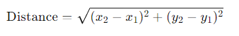
We used pyLDAvis (Sievert & Shirley, 2014) to perform multidimensional scaling on the resulting topics. As a result, each topic can be represented by its coordinates ((x, y)) in a two-dimensional space. The Euclidean distance between two points is given by:
Each document ( D ) is represented by a vector ( w_D ) of 50 topic weights
Using these weights, we can calculate the topic distance between two documents.
Explanation with Example
Let’s break down the explanation and provide an example step by step:
1. Estimating a Topic Model with Gensim
What is Gensim?
Gensim is a Python library for topic modeling, document indexing, and similarity retrieval with large corpora. It’s known for its efficiency and ease of use in building topic models, among other functionalities.
Topic Modeling and LDA
Topic modeling is a method for uncovering the hidden thematic structure in a large collection of documents. Latent Dirichlet Allocation (LDA) is a popular topic modeling technique that represents documents as mixtures of topics and topics as mixtures of words.
Example:
Imagine you have a collection of news articles. You want to discover the main themes (topics) within these articles without reading each one individually.
2. Choosing the Number of Topics and Data Preparation
Perplexity and Interpretability
- Perplexity: A measure of how well a probability model predicts a sample. Lower perplexity indicates a better generalization performance.
- Interpretability: How meaningful and coherent the resulting topics are to humans.
You evaluated different models and chose an LDA model with 50 topics, as this number provided a good balance between low perplexity and high interpretability.
tf-idf Representation
- tf-idf (term frequency-inverse document frequency): A statistical measure used to evaluate how important a word is to a document in a collection or corpus. It helps in filtering out common but less informative words.
Example:
In your news articles, words like “the”, “is”, and “and” are extremely common and not very informative. Words like “election”, “pandemic”, and “technology” are less common but more informative. tf-idf helps in emphasizing these important words.
3. Filtering Words
You also filtered out extremely common and uncommon words to improve the model’s performance.
Example:
Common words filtered out: “the”, “is”, “and”.
Uncommon words filtered out: Rare words that appear in only one or two documents.
4. Visualizing Topics with pyLDAvis
pyLDAvis
pyLDAvis is a Python library for interactive topic model visualization. It uses multidimensional scaling (MDS) to represent topics in a 2D space, making it easier to explore and interpret the topics.
Example:
After running the LDA model, you use pyLDAvis to plot the topics. Each topic is represented as a point in a 2D space, where the distance between points represents the dissimilarity between topics.

5. Representing Documents with Topic Weights
Each document is represented by a vector of 50 topic weights. This vector indicates the document’s distribution over the 50 topics.
Example:
If a document is about politics and technology, its vector might look like:
where the weights represent the proportions of different topics.
6. Calculating Topic Distance Between Documents
Using the topic weights, you can calculate the Euclidean distance between two documents in the topic space. The Euclidean distance between two points ((x_1, y_1)) and ((x_2, y_2)) is given by:
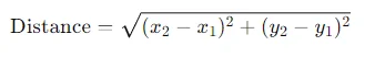
Example:
Let’s say we have two documents:

The distance between these two documents can be calculated using the Euclidean distance formula in a 50-dimensional space.
Summary
By using Gensim for LDA topic modeling, you can identify the main themes in your document collection. With pyLDAvis, you can visualize these themes in a 2D space, and by representing documents as vectors of topic weights, you can compute the distances between documents, providing insights into their thematic similarities and differences.

Category and Tag Distance
Another more recent approach is the use of word embeddings to capture the aggregate inter-document difference by considering the Wasserstein metric, which describes the minimum effort to make two documents similar. This is called the Word Mover’s Distance (WMD). The great benefit of this method is that it is not sensitive to non-overlapping document vocabularies. We use a word vector model pre-trained on the NLCOW14 corpus (see Tulkens et al., 2016; Schäfer & Bildhauer, 2012), applied using Gensim.
In addition, we also have human-labeled tags as proxies for the topics and the newspaper sections for each article as proxies for the categories. We apply the word distance derived from the word vector trained on the NLCOW14 corpus to these tags and categories.
Category and Tag Distance: Detailed Explanation
Word Embeddings and Word Mover’s Distance (WMD)
Word Embeddings:
- Word embeddings are a type of word representation that allows words to be represented as vectors in a continuous vector space. Words with similar meanings are positioned closer together in this space.
- These embeddings are often pre-trained on large text corpora using methods like Word2Vec, GloVe, or Fast Text.
Word Mover’s Distance (WMD):
- WMD is a metric used to measure the distance between two documents by calculating the minimum cumulative distance that words from one document need to travel to match the words from another document.
- It uses the concept of the Wasserstein distance, which is a measure of the effort required to transform one distribution into another.
Key Benefits of WMD:
- Insensitive to Non-Overlapping Vocabularies: Unlike traditional methods that require exact word matches, WMD can compare documents with completely different vocabularies by using word embeddings to find semantic similarities between words.
Implementation:
- Pre-trained Word Vector Model: We use a word vector model pre-trained on the NLCOW14 corpus. This corpus is a large collection of web texts, providing a rich set of word vectors for our analysis.
- Gensim: Gensim is a Python library for topic modeling and document similarity analysis, which includes functions to calculate WMD using pre-trained word vectors.
Example:
Imagine we have two documents:

- Document A: “The cat sat on the mat.”
- Document B: “A feline rested on the rug.”
Using WMD, we can measure the semantic similarity between these two documents by calculating the minimum distance the words “cat” and “feline”, “sat” and “rested”, “mat” and “rug” need to travel in the vector space to align with each other.
Human-Labeled Tags and Newspaper Sections
In addition to WMD, we also use human-labeled tags and newspaper sections to further analyze the documents.
Human-Labeled Tags:
- Tags are labels assigned to articles that capture key topics or themes. For example, a news article might be tagged with “politics”, “election”, and “government”.
- These tags serve as proxies for the topics discussed in the articles.
Newspaper Sections:
- Newspaper sections are the categories under which articles are published, such as “sports”, “business”, “entertainment”, etc.
- These sections serve as proxies for broader categories of content.
Using Word Embeddings for Tags and Categories:
- We apply the same word distance approach derived from the word vector model pre-trained on the NLCOW14 corpus to the tags and newspaper sections.
- By representing tags and categories as vectors, we can calculate the semantic distance between them, similar to how we compare entire documents.
Example:
Suppose we have two articles:
- Article A: Tagged with “technology”, “innovation”, “startup”.
- Article B: Tagged with “business”, “entrepreneurship”, “investment”.
Using the pre-trained word vectors, we can compute the semantic distance between these tags to determine how similar the articles are in terms of their topics.
Summary
By combining word embeddings with the Word Mover’s Distance, and leveraging human-labeled tags and newspaper sections, we can effectively measure the semantic distance between articles. This approach allows for a nuanced comparison that is not limited by vocabulary differences, providing a richer understanding of the content and its categorization.

3.2.3. Ratio of Politically Relevant Content
Explanation:
To estimate how politically relevant an article is, we start by identifying words closely related to ‘politiek’ (which means ‘politics’ or ‘political’ in Dutch). This is done using a word vector model, a type of natural language processing technique that represents words in a continuous vector space where semantically similar words are closer together.
Example:
- Constructing the Word List:
- Suppose our word vector model suggests that words like ‘government’, ‘election’, ‘policy’, ‘minister’, ‘legislation’, etc., are closely related to ‘politiek’.
- We manually add some other words we believe are relevant, such as ‘parliament’, ‘democracy’, and ‘campaign’.
- Comparing with Article Text:
- For an article about a new city park, we count the occurrences of the words from our list within the article. If very few or none of these words appear, the article is considered to have a low ratio of politically relevant content.
- Conversely, an article discussing a recent election might have many of these words, indicating a high ratio of politically relevant content.

3.2.4. Tone Distance
Explanation:
Tone distance involves assessing the sentiment (polarity) and subjectivity of an article. This is done using the Pattern package, which is capable of determining these values for Dutch-language text. Each article is placed in a two-dimensional sentiment space based on its polarity (from -1 for very negative to +1 for very positive) and subjectivity (from 0 for very objective to +1 for very subjective).
Example:
- Sentiment Analysis:
- For an article about a tragic event, the Pattern package might return a tuple like (-0.8, 0.5), indicating a highly negative and somewhat subjective tone.
- For an article about a successful community project, the tuple might be (0.7, 0.2), indicating a positive and relatively objective tone.
- Two-Dimensional Sentiment Space:
- Plotting these tuples, we can visualize where each article lies in terms of sentiment and subjectivity.
- Articles close together in this space are similar in tone, while those far apart have different tones.

3.3. Diversity Evaluation
Explanation:
To evaluate diversity, we calculate pairwise distances between articles and describe their distributions for each recommender system. Formal diversity measures like Rao’s quadratic entropy and Shannon entropy are used. Rao’s quadratic entropy considers the proportion and distance metric (cosine similarity of word vectors), whereas Shannon entropy measures category distribution without considering the relative distances between articles.
Example:
- Rao’s Quadratic Entropy:
- If our document categories are ‘Politics’, ‘Health’, ‘Entertainment’, etc., we compute the proportion of articles in each category.
- We calculate the cosine similarity between word vectors of the main section titles of these articles.
- For instance, if ‘Politics’ articles are very similar to each other but different from ‘Health’ articles, the diversity score will reflect these distances.
- We modify the proportions to favor niche categories by using
- ensuring less common categories contribute more to the diversity score.
- Shannon Entropy:
- Shannon entropy is calculated as
- of articles in each category.
- For example, if we have a balanced distribution across ‘Politics’, ‘Health’, and ‘Entertainment’, the entropy will be high, indicating good diversity.
- However, even if a small category like ‘Science’ is underrepresented, Shannon entropy might still indicate high diversity, potentially missing out on the lack of niche representation.
By using these measures, we can evaluate how well a recommender system promotes diverse content, ensuring a wide representation of topics and tones.